Quick-Start Guide • mvbcf

To get started quickly, and test everything is working properly, here is a simple example showing how to use the package with the default hyper-parameter settings. For more details on the hyper-parameters and other guides, see the other examples.

Fitting The Model

#Load the mvbcf package
library(mvbcf)

#set seed
set.seed(101)

#Create some synthetic data
#number of observations
n<-500
#number of covariates
p<-5

#matrix of covariates
X<-matrix(runif(n*p), nrow=n)

#The outcome under control for y1 and y2
mu1<-3*X[,1]-4*X[,3]^2
mu2<-4*X[,1]+1*X[,3]^2-2*X[,5]

#The effect of receiving treatment on y1 and y2
tau1<-1*X[,1]
tau2<-0.6*X[,1]

#The probability of receiving treatment (true propensity score)
true_propensity<-(X[,2]+X[,3])/3

#Treatment status
Z<-rbinom(n, 1, true_propensity)

#The observed outcomes
y1<-mu1+Z*tau1+rnorm(n, 0, 1)
y2<-mu2+Z*tau2+rnorm(n, 0, 1)

Y<-cbind(y1, y2)

mvbcf_mod <- run_mvbcf(X,
                       Y,
                       Z,
                       X)

Check Convergence

Quick look at convergence of posterior of $\Sigma_{1,1}$ and $\Sigma_{2,2}$ (The residual variance corresponding to outcome variables $y_{1}$ and $y_{2}$ ).

plot(mvbcf_mod$sigmas[1,1,], type="l", ylab="Sigma11 Samples")

plot(mvbcf_mod$sigmas[2,2,], type="l", ylab="Sigma22 Samples")

Look at Average Treatment Effect (ATE) Posterior

Histogram of posterior samples of ATE (Average Treatment Effect) for $y_{1}$ and $y_{2}$ .


hist(colMeans(mvbcf_mod$predictions_tau[,1,]),
     xlab="Tau1 ATE Samples",
     main="Histogram of Posterior Samples")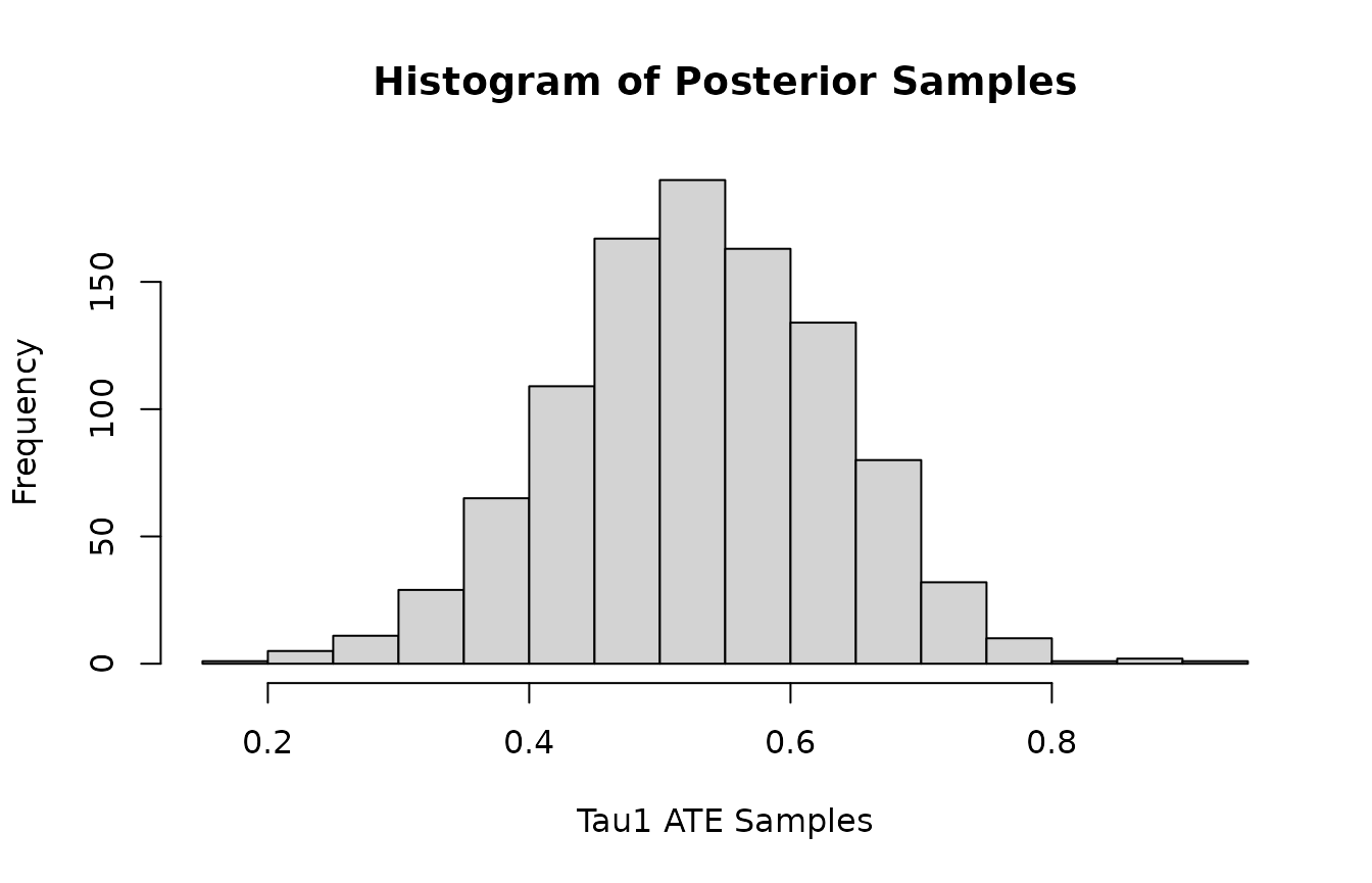


hist(colMeans(mvbcf_mod$predictions_tau[,2,]),
     xlab="Tau2 ATE Samples",
     main="Histogram of Posterior Samples")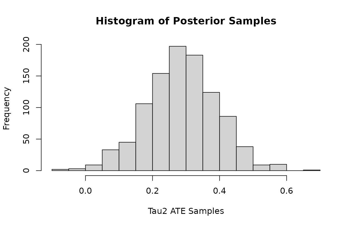

Look at Model Predictions

Get predicted $\mu$ , $\tau$ , and $y$ predictions, then compare with ground truth.


mu1_preds<-rowMeans(mvbcf_mod$predictions[,1,])
mu2_preds<-rowMeans(mvbcf_mod$predictions[,2,])

tau1_preds<-rowMeans(mvbcf_mod$predictions_tau[,1,])
tau2_preds<-rowMeans(mvbcf_mod$predictions_tau[,2,])

y1_preds<-rowMeans(mvbcf_mod$predictions[,1,]+Z*mvbcf_mod$predictions_tau[,1,])
y2_preds<-rowMeans(mvbcf_mod$predictions[,2,]+Z*mvbcf_mod$predictions_tau[,2,])


plot(mu1, mu1_preds, main="Predicted vs. True Values", xlab="Mu1", ylab="Mu1 Predictions")
abline(0,1)


plot(tau1, tau1_preds, main="Predicted vs. True Values", xlab="Tau1", ylab="Tau1 Predictions")
abline(0,1)


plot(y1, y1_preds, main="Predicted vs. True Values", xlab="y1", ylab="y1 Predictions")
abline(0,1)


y1_residuals<-y1-y1_preds
qqnorm(y1_residuals)
qqline(y1_residuals)